OFFSET Function

MS Excel: How to use the OFFSET Function (WS)

This Excel tutorial explains how to use the Excel OFFSET function with syntax and examples.

Description

The Microsoft Excel OFFSET function returns a reference to a range that is offset a number of rows and columns from another range or cell.

The OFFSET function is a built-in function in Excel that is categorized as a Lookup/Reference Function. It can be used as a worksheet function (WS) in Excel. As a worksheet function, the OFFSET function can be entered as part of a formula in a cell of a worksheet.

Syntax

The syntax for the OFFSET function in Microsoft Excel is:

OFFSET( range, rows, columns, [height], [width] )

Parameters or Arguments

range

The starting range from which the offset will be applied.

rows

The number of rows to apply as the offset to the range. This can be a positive or negative number.

columns

The number of columns to apply as the offset to the range. This can be a positive or negative number.

height

Optional. It is the number of rows that you want the returned range to be. If this parameter is omitted, it is assumed to be the height of range.

width

Optional. It is the number of columns that you want the returned range to be. If this parameter is omitted, it is assumed to be the width of range.

Returns

The OFFSET function returns a reference.

Applies To

• Excel 2016, Excel 2013, Excel 2011 for Mac, Excel 2010, Excel 2007, Excel 2003, Excel XP, Excel 2000

Type of Function

• Worksheet function (WS)

Example (as Worksheet Function)

Let's look at some Excel OFFSET function examples and explore how to use the OFFSET function as a worksheet function in Microsoft Excel:

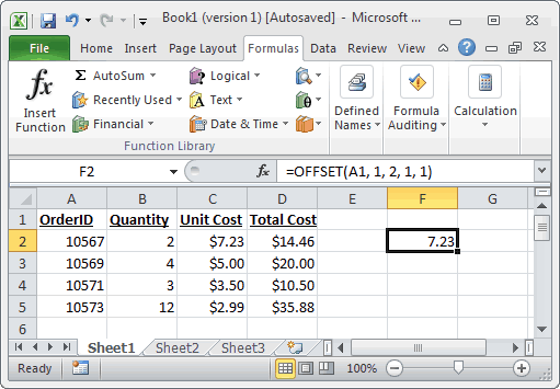
Based on the Excel spreadsheet above, the following OFFSET examples would return:

=OFFSET(A1, 1, 2, 1, 1)
Result: reference to cell C2   (and thus would display $7.23)

=OFFSET(C3, -1, -2, 1, 1)
Result: reference to cell A2   (and thus would display 10567)